Neural Networks in Carbon and Code
02 March 2017

The artificial neural network is a powerful programming paradigm that has achieved some impressive feats in recent years. The algorithms in this style are based on an analogy to the information pathways in biological nervous systems like the brain. But how alike are artificial and biological neural networks? And what elements must be alike for the metaphor to hold? This is a big topic and I’ve only just scratched the surface, but if you’re willing to brave my possible misinterpretations I’ll share what I’ve learned so far.
Neurons in Carbon
A neuron is a cell capable of transmitting information through electrical and chemical signals. These tiny cells are the fundamental building blocks of the brain and the entire nervous system. There are some specialised input neurons in sensory organs which convert information from the world (touch, sound, light) into electrical impulses and specialised output neurons that convert electrical impulses from the nervous system into muscle movement. The vast majority of neurons in your body however are simply connected to other neurons.
In a neuron, informations flows in a single direction. Left to right in the image below. The main body of the cell collects information from other neurons, via synapses. A synapse is a microscopic gap between the output end of one neuron and the input end of another, sometimes itself. This gap is jumped when enough charge is built up on the input end. Synapses can be of varying strengths, possible due to repeated stimulation.
Neurons have long tree-like branches called dendrites stretching outward from the cell body. Most of the cell’s synapses are connected along these branches. The neuron’s charge is the sum of all of the charges from the neurons upstream. A single neuron can have millions of synaptic connections with others. When the sum of inputs to a neuron reaches the threshold, a charge is released down its tail, called an axon. Finally there is another series of branches each ending in a small bulb called an axon terminal. These terminals connect to the body or dendrites of other neurons to form more synapses and so the flow of information continues.

Neurons in code
In the computational model of a neuron there is no need for the complex physical structures. We simply model the flow of information. As such, a neuron is just a value resulting from its relations to other neurons. The diagram below shows the calculation of a single neuron value from it’s upstream inputs. There are three inputs to this neuron connected via synapses of varying strengths. We can think of the synapse strengths as coefficients which moderate the relevance of any upstream neurons.
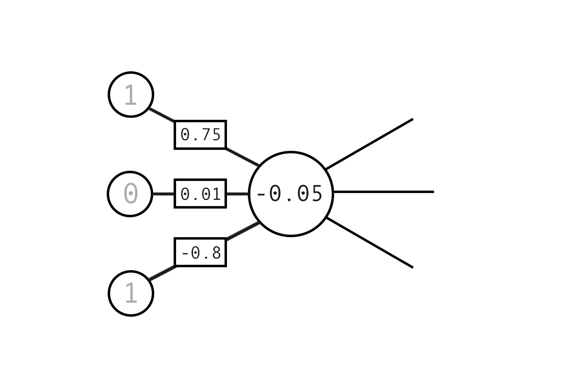
Computational neurons are the sum of their connected inputs multiplied by their synaptic strength. As such, the example below is calculated as:
1 * 0.75 +
0 * 0.01
1 * -0.8
= -0.05
This new neuron can then feed out via further synapses to other neurons.
There are some obvious functional differences here between biology and computation. The biological neurons have a threshold value which when reached results in immediate firing. This means that a biological neuron is either on or off, while the computational neuron can take on analog values. It is possible to include a threshold and binary values in the computational model (the classic perceptron is an example of this) but these tend to be impossible to train as small changes to weights can cause results to flip. It is also worth noting that although a biological neuron is either on or off, the effect of analog signals are produced by varying frequencies of firing.
Emergence and connectionism
A neuron in and of itself is not enough to constitute thinking. How then can we make sense of the incredible feats of cognition of which the brain or even from artifical neural networks are capable? One proposed solution is connectionism. According to connectionism, mental phenomena emerge from the connections between many simple units. This model posits that learning involves the adjustment of connection strenghts and attibutes learning, understanding and memory this process.
In biological neural networks the adjustment of connection is commonly attributed to repeated patterns of firing, the theory goes that synapses strengthen when used and atrophy when left dormant. In artificial neural nets we adjust synapse strengths with an algorithm called backpropagation which I’ll demostrate in code examples later on.
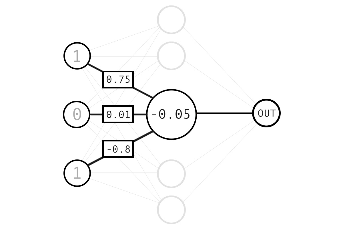
The diagram below shows the structure of a simple network of neurons which we’re about to code.
Coding a neural network
The connectionist model, regardless of its ultimate “truth”, has had some incredible successes as a way of programming. It is worth remembering however, that other models of cognition such as computationalism have also had successes in producing apparantly intelligent behaviour. With that said, there is something truly mindbending about neural networks, they seem to defy reason.
All the examples that follow will be in clojure. If that’s not your cup of tea, I recommend A Neural Network in 11 lines of Python (Part 1) by Trask. It deals with the same problem in a more orthodox pythonic style.
Lets start by establishing some training data.
(def training-data
   ;; input => output
   [ [0 0 1]   [0]
     [0 1 1]   [1]
     [1 0 1]   [1]
     [1 1 1]   [0] ])
We can easily extract the input and output like so.
(def training-input
  (take-nth 2 training-data))

(def training-output
  (take-nth 2 (rest training-data)))
We want to initialise our synapses as random values between -1 and 1.
(def random-synapse #(dec (rand 2)))
We’ll need a synapse weight from every neuron in the input layer to every one in the output layer. We’ll represent this as a matrix of size [number-of-inputs, number-of-outputs]. It’s usually better to create reusable functions so my solution is matrix-of which works a bit like clojure.core’s repeatedly.
(defn matrix-of [function shape]
  (repeatedly (first shape)
    (if (empty? (rest shape))
      function
      #(matrix-of function (rest shape))))
Now our code describes it’s function to the reader.
(matrix-of random-synapse [3 5])
The synapses are mutable so we’ll want to use atoms.
(def synapses-0
  (atom (matrix-of random-synapse [3 5])))

(def synapses-1
  (atom (matrix-of random-synapse [5 1])))
Activation/Deactivation
For our network to function over multiple layers of neurons we need a way of keeping values within 0 and 1. To solve this we’ll need a non-linear activation function. This is probably best demonstrated by example.
REPL> (activate 0)
;; => 0.5
REPL> (activate 1)
;; => 0.7310585786300049
REPL> (activate -5)
;; => 0.0066928509242848554
REPL> (activate 10)
;; => 0.9999546021312976
Here I’m going to use the standard logistic function but tanh and other sigmoidal curves will also work.
(defn activate
  "Standard logisitic function"
  [x] (/ 1 (+ 1 (matrix/exp (- x)))))

(defn deactivate
  "Reverse activation operation"
  [x] (* x (- 1 x)))
Feed forward
We can calculate the neurons of the next layer very simply. We saw before that the value of a neuron is equal to the sum of it’s inputs multiplied by their synaptic weights. We could iterate this way to get our result, but this can be achieved even more elegantly with the matrix dot product.
(defn step-forward
  "For each step in feed forward, the new layer of neurons
  are a function of the previous layer and it's synapses"
  [neurons synapses]
  (activate (matrix/dot neurons synapses)))
The above works fine, but I think a single feed forward function which carries out an arbitrary level of layers would be nicer.
(defn feed-forward
  [input & synapses]
  (case (count synapses)
    0 input ; if no synapses return just the input
    1 (step-forward input @(first synapses))
    ;; otherwise recur
    (apply
     feed-forward
     (into [(step-forward input @(first synapses))]
           (rest synapses)))))
Now all the required information can be applied as arguments to the feed-forward function.
(feed-forward training-input @synapses-0 @synapses-1)
And we get our result! The only problem is that our result is about as good as flipping a coin.
Calculating the Error
Our network is functional, but how did it do? We can measure the total error pretty easily by finding the difference between our training outputs and the return value of our feed forward network.
(defn errors [training-outputs real-outputs]
  (- training-outputs real-outputs))

(defn mean-error [numbers]
  (let [absolutes (map abs (flatten numbers))]
    (/ (apply + absolutes) (count absolutes))))

REPL> (mean-error
        (error
          training-output
          (feed-forward training-input @synapses-0 @synapses-1)))
;; => 0.496748102
With our current untrained network the mean error should be somewhere around 0.5.
Training the Network
How can we turn our functional, but utterly abysmal network into a powerful predictor? Perhaps surprisingly, all we change from here on out is the synapse strengths, in other words the intelligence of the system emerges entirely from the connections between neurons, not the neurons themselves. This process is a bit like tuning a piano.
The process of tuning involves calculating the effects of each synapse on the system’s total error and adjusting to reduce the error.
(defn output-deltas [targets outputs]
  (* (deactivate outputs)
     (- targets outputs)))

(defn hidden-deltas [output-deltas neurons synapses]
  (* (matrix/dot output-deltas (matrix/transpose synapses))
     (deactivate neurons)))
These changes we calculate can then be applied to the synapses in the system.
(defn apply-deltas [synapses neurons deltas learning-rate]
  (+ synapses
     (* learning-rate
        (matrix/dot (matrix/transpose neurons) deltas))))
Then, all we need to do is reset the synapses values with the deltas applied.
(reset! synapses-0
  (apply-deltas @synapses-0 training-input hidden-delta 1))

(reset! synapses-1
  (apply-deltas @synapses-1 hidden-layer output-delta 1))
We can wrap this up in a single training function.
(defn train
  "Train the network and return the error"
  [training-input training-output]
  (let [
        hidden-layer (step-forward training-input @synapses-0)
        output-layer (step-forward hidden-layer @synapses-1)
        output-delta (output-deltas training-output output-layer)
        hidden-delta (hidden-deltas output-delta hidden-layer @synapses-1)
        output-error (errors training-output output-layer)
        ]
    (do
      (swap! synapses-1
             #(apply-deltas % hidden-layer output-delta 1))
      (swap! synapses-0
             #(apply-deltas % training-input hidden-delta 1))
      (mean-error output-error)
      )))

;; We need to do this a lot of times to get good results.
(dotimes [i 10000]
  (train training-input training-output))

;; Check results
(feed-forward training-input synapses-0 synapses-1)
Artificial neural networks are fascinating. Their apparant intelligence seems to surprise even those who understand their mathematical foundation. Whether or not these algorithms really function “like a brain” is still an open question. Certainly there are functional differences between biological neurons and their computational simulacra, though the ontological consequences of these are difficult to comprehend as neither system’s emergent qualities can be easily explained by their simple parts. No doubt I still have a lot to learn in this area.
The code for from this post can be found here.
Reading List
- Clarke, Arthur Charles. The Nine Billion Names of God. New American Library, 1974.